Support vector machines

The 3 parts of an SVM

The SVM consists of 3 "tricks" combined to give one of the most influential and arguably state-of-the-art machine learning algorithm.  The 3rd, "kernel trick" is what gives SVM its power.

During the talk I will refer to Cortes and Vepnik's 1995 paper.

1. A linear classification problem, ie, separating a set of data points by a straight line / plane.  This is very simple.
2. Transforming the primal optimization problem to its dual via Lagrangian multipliers.  This is a standard trick that does not result in any gain / loss in problem complexity.  But the dual form has the advantage of depending only on the inner product of input values.
3. The kernel trick that transforms the input space to a high dimensional feature space.  The transform function can be non-linear and highly complex, but it is defined implicitly by the inner product.

1. The maximum-margin classifier

The margin is the separation between these 2 hyper-planes:

 $ \bar{w}^* \cdot \bar{x} = b^* + k $

 $ \bar{w}^* \cdot \bar{x} = b^* - k $

so the maximum margin is given by:

 $ m^* = \frac{2k}{|| \bar{w}^* ||} $

The optimization problem is to maximize $m^*$, which is equivalent to minimizing:
$$ \max (m^*) \Rightarrow \max_{\bar{w}} (\frac{2k}{ || \bar{w} || })
\Rightarrow \min_{\bar{w}} (\frac{ || \bar{w} || }{2k})  \Rightarrow \min_{\bar{w}} ( \frac{1}{2} \bar{w} \cdot \bar{w} ) $$subject to the constraints that the the hyper-plane separates the + and - data points:
$$ \bar{w} \cdot (y_i \bar{x_i} ) \ge 1 + y_i b $$

This is a convex optimization problem because the objective function has a nice quadratic form $\bar{w} \cdot \bar{w} = \sum \bar{w_i}^2$ which has a convex shape:

2. The Lagrangian dual

The Lagrangian dual of the maximum-margin classifier is to maximize:
$$ \max_{\bar{\alpha}} ( \sum_{i=1}^{l} \alpha_i - \frac{1}{2} \sum_{i=1}^{l} \sum_{j=1}^{l} \alpha_i \alpha_j y_i y_j \bar{x_i} \cdot \bar{x_j} ) $$subject to the constraints:
$$ \sum_{i=1}^l \alpha_i y_i = 0, \quad  \alpha_i \ge 0 $$
Lagrangian multipliers is a standard technique so I'll not explain it here.

Question:  why does the inner product appear in the dual?  But the important point is that the dual form is dependent only on this inner product $(\bar{x_i} \cdot \bar{x_j})$, whereas the primal form is dependent on $(\bar{w} \cdot \bar{w})$.  This allows us to apply the kernel trick to the dual form.

3. The kernel trick

A kernel is just a symmetric inner product defined as:
$$ k(\mathbf{x}, \mathbf{y}) = \Phi(\mathbf{x}) \cdot \Phi(\mathbf{y}) $$By letting $\Phi$ free we can define the kernel as we like, for example, $ k(\mathbf{x}, \mathbf{y}) = \Phi(\mathbf{x}) \cdot \Phi(\mathbf{y}) = (\mathbf{x} \cdot \mathbf{y} )^2 $.

In the Lagrangian dual, the dot product $(\bar{x_i} \cdot \bar{x_j})$ appears, which can be replaced by the kernel $k(\bar{x_i}, \bar{x_j}) = (\Phi(\bar{x_i}) \cdot \Phi(\bar{x_j}))$.

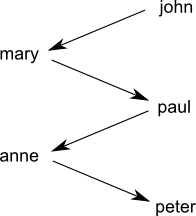
Doing so has the effect of transforming the input space $\mathbf{x}$ into a feature space $\Phi(\mathbf{x})$, as shown in the diagram:

But notice that $\Phi$ is not explicitly defined;  it is defined via the kernel, as an inner product.  In fact, $\Phi$ is not uniquely determined by a kernel function.

This is a possible transformation function $\Phi$ for our example:
$$ \Phi(\mathbf{x}) = (x_1^2, x_2^2, \sqrt{2} x_1 x_2) $$It just makes $ \Phi(\mathbf{x}) \cdot \Phi(\mathbf{y}) $ equal to $ (\mathbf{x} \cdot \mathbf{y} )^2 $.

Recall that the inner product induces a norm via:

$ ||\mathbf{x}|| = \sqrt{\mathbf{x} \cdot \mathbf{x}} $

and the distance between 2 points x and y can be expressed as:

$ d(\mathbf{x},\mathbf{y})^2 = || \mathbf{x - y} ||^2 = \mathbf{x} \cdot \mathbf{x} + \mathbf{y} \cdot \mathbf{y} - 2 \mathbf{x} \cdot \mathbf{y}$

Thus, defining the inner product is akin to re-defining the distances between data points, effectively "warping" the input space into a feature space with a different geometry.

Some questions:  What determines the dimension of the feature space?  How is the decision surface determined by the parameters $\alpha_i$?

Hilbert Space

A Hilbert space is just a vector space endowed with an inner product or dot product, notation $\langle \mathbf{x},\mathbf{y}\rangle$ or $(\mathbf{x} \cdot \mathbf{y})$.

The Hilbert-Schmidt theorem (used in equation (35) in the Cortes-Vapnik paper) says that every self-adjoint operator in a Hilbert space H (which can be infinite-dimensional) forms an orthogonal basis of H.  In other words, every vector in space H has a unique representation of the form:

$$ \mathbf{x} = \sum_{i=1}^\infty \alpha_i \mathbf{u}_i $$This is called a spectral decomposition.

*  *  *

As a digression, Hilbert spaces can be used to define function spaces.  For example, this is the graph of a function with an integer domain:

with values of $f(1), f(2), f(3), ... $ on to infinity.  So, each graph corresponds to one function.

Imagine an infinite dimensional space.  Each point in such a space has dimensions or coordinates $(x_1, x_2, ... )$ up to infinity.  So we can say that each point defines a function via
$$f(1) = x_1, \quad f(2) = x_2, \quad f(3) = x_3, ... $$
In other words, each point corresponds to one function.  That is the idea of a function space.  We can generalize from the integer domain ($\aleph_0$) to the continuum ($2^{\aleph_0}$), thus getting the function space of continuous functions.

End of digression :)

Introducing Genifer, 2012

I started working on AGI in 2004, and my greatest "achievement" up to 2012 (8 years) is the invention of a new logic.  All my work thus far is focused on the thinking aspect of AGI, deferring the aspects of planning and acting.

Concept composition logic

Consider a complex sentence:
     "John walks to church slowly, thinking about Turing"

It can be decomposed into:

1. "John walks to church"
2. "John walks slowly"
3. "John walks thinking about Turing"

Using the Genifer GUI (github code is here) we can manually create a graph that represent the sentence structure as follows:

The GUI automatically generates a "factorization" formula of the graph.

The key idea of the graph is that if a word A modifies word B, we create an arrow $A \multimap B$.  More than 1 word can modify a target, but each word can only modify 1 target.  This ensures that the result is a tree, and can be expressed as a sum of products, using $+$ and $\times$.

We can use the distributive law of multiplication to expand the factorized formula.

A problematic case:  If we translate these 2 sentences into logic:

1. "John gives the ball to Mary"  and
2. "John gives $2 to Kevin"

After factorizing and expanding we get:

1. john gives to mary
2. john gives the ball
3. john gives to kevin
4. john gives $2

so it may be confused that John gives $2 to Mary.  But I reckon that the distributive law is not the real cause of the error.  The error arises because the 2 "johns" are the same John but the 2 "gives" are different instances of giving.

Variable-free logic

This is an example of the logical definition of "downstairs" from the SUMO ontology:

On the left side is the logic formula, on the right the English translation.  As you can see from the translation, it uses a lot of "$n^{th}$ objects" which are logic variables.  But notice that all these variables invariably belong to some classes (such as "building_level").  So we can just do without variables and directly use ontology classes for matching.

For example:
    "All girls like to dress pretty"
    "Jane is a girl"
implies "Jane likes to dress pretty".

In logic the steps would be:
    girls like to dress pretty
    jane $\in$ girls
    $\Rightarrow$ jane likes to dress pretty
because the "girl" atom in both formulas match, so "jane" is substituted into the conclusion.

Parsing of natural language

This is an example parse tree of an English sentence:

A simple grammar rule is:
   "A noun phrase (NP) followed by a verb phrase (VP) is a sentence (S)".

In classical AI, which uses first-order predicate logic, we have to parse the English sentence to obtain the parse tree (syntax parsing), and then translate the parse tree into logic (semantic parsing).  The final logic formula would be like:  loves(john, mary).  The semantic parsing process is complicated and involves using $\mathbf{\lambda}$-calculus to represent sentence fragments.

In our new logic we can just write:
    NP $\circ$ VP $\in$ S

And we have these as data:
    loves $\circ$ mary $\in$ VP                           "loves mary is a verb phrase"
    john $\in$ NP                                          "john is a noun phrase"
    $\Rightarrow$ john $\circ$ loves $\circ$ mary $\in$ S             "john loves mary is a sentence"

Thus, we have achieved both syntax and semantic parsing using just one logic rule (for each grammar rule)!  This is a tremendous improvement over classical AI.  (But I would add that my new logic is just a kind of syntactic sugar for classical logic.  Nevertheless, the syntactic sugar in this case results in very significant simplification of implementation, whereas the classical approach may be so complicated as to be unusable.)

In summary, my innovation provides a new algebraic format of logic that can change our perspectives and open up new algorithmic possibilities.

Introduction to machine learning

[ I'd be giving a talk to introduce Genifer to some Hong Kong people interested in machine learning.  This is the presentation material. ]

Computer vision

Some of you have told me that you're interested in computer vision, so I'll start with visual perception.

The first thing to know is that the computer vision problem is theoretically already solved.  There is no mystery in machine vision:

When we look at a scene, what we have is a image which is a projection of the scene's objects onto a retina.  The mathematics of such a projection is completely specified by projective geometry, with some changes due to occlusion (blocking of light rays).  The machine vision problem is to compute the inverse of the projection, ie, $f^{-1}$.

Of course you also need a way to represent physical objects in the scene.  There are many data structures designed for that purpose, with Clifford algebra (or geometric algebra) being a more mathematical technique.

So why is the vision problem still unsolved?  I guess it's mainly because researchers try to solve the problem using relatively simple or "clever" mathematical tricks instead of really solving every step along the chain of $f^{-1}$.  To do this would require a large scale project, probably beyond the reach of a single professor with a few grad students.

And if someone takes the trouble to solve vision completely, they might just as well tackle the problem of general intelligence (AGI)!

2 type of machine learning

All of machine learning is a search for hypotheses in the hypothesis space.  The resulting hypothesis may not be necessarily correct, but it is the best given the data and based on some criteria ("scores").

There are 2 major paradigms of machine learning:

1. logic-based learning
   -- hypotheses are logic formulas
   -- search in the space of logic formulas
   -- uses classical AI search techniques
2. statistical learning (including neural networks)
   -- emerged in the 1990s
   -- data points exist in high dimensional space
   -- use geometric structures (planes or surfaces) to cut the space into regions
   -- learning is achieved through parameter learning
   -- includes neural networks, support vector machines, ...

Neural networks

This is a neuron:

A neuron receives input signals on its dendrites from other neurons.  When the sum of the inputs exceeds a certain threshold, an action potential is fired and propagates along the axon, that reaches other neurons.

Equation of a single neuron

The equation of a neuron is thus:

$$ \sum w_i x_i \ge \theta $$

where the $x_i$'s are inputs, the $w_i$'s are called the weights, $\theta$ is the threshold.

Graphically, each neuron is a hyper-plane that cuts the hyperspace into 2 regions:

Thus imagine multiple neurons chopping up hyperspace into desired regions.

Back-propagation

Back-propagation is a technique invented in the 1970s to train a multi-layer neural network to recognize complex, non-linear patterns.

This is the step function of the inequality $\sum w_i x_i \ge \theta$:

This is replaced by the smooth sigmoid function:

So the equation now becomes:  $\Phi( \sum w_i x_i ) \ge \theta$.

Recall that in calculus, we have the chain rule for differentiation:

$$ D \; f(g(x)) = f ' (g(x)) \cdot g'(x) $$

(The derivative does not exist for the step function because it is not smooth at the threshold point).

Imagine each layer of the neural network as a function $f_i$.  So the chain rule allows us to propagation the error ($\Delta x$) from the lowest layer ($f_1$) to the highest layer ($f_n$):

$$ f_n(f_{n-1}( ... ... f_2(f_1(\Delta x)) ... ) $$

(The formula is just a figurative illustration).  So we can gradually tune the parameters of the neurons in each layer to minimize the error.

Support vector machines

[ See next blog post. ]

Logical / relational learning

This is an example (correct) hypothesis:

$ uncle(X, Y) \leftarrow parent(Z, Y) \wedge brother(Z, X) $

This hypothesis would be too general:

$ uncle(X, Y) \leftarrow $   parent(Z, Y)  $ \wedge brother(Z, X) $

Whereas this one is too specific:

$ uncle(X, Y) \leftarrow parent(Z, Y) \wedge brother(Z, X) \wedge has\underline{ }beard(X) $

Logical inductive learning searches in the space of logic formulas, structured by this general-specific order (also known as subsumption order).

An order (<, Chinese 序) creates a structure called a lattice (Chinese 格).  This is an example of a lattice:


This is another example of a lattice:



Sometimes we use $\top$ to denote the top element (ie, the most general statement, meaning "everything is correct"), and $\bot$ to denote the bottom element (ie, the most specific statement, meaning "everything is false").

About logic, and how to do it fast

In this article I will talk about 2 things:

1. The difference between propositional and predicate logic
2. How to make logic inference fast

What is the difference between propositional logic and predicate logic?

For example, "rainy", "sunny", and "windy" are propositions.  Each is a complete sentence (consider, eg "it is sunny today") that describe a truth or fact, and we assume the sentence has no internal structure.

In contrast, predicate logic allows internal structure of propositions in the form of predicates and functions acting on objects.  For example:  loves(john, mary)  where "loves" is a predicate and "john", "mary" are objects.  They are called first-order objects because we can use the quantifiers $\forall X, \exists X$ to quantify over them.  Second-order logic can quantify over predicates and functions, and so on.

An example of a propositional machine learning algorithm is decision tree learning.  This is the famous example:

All the entries are given as data, the goal is to learn to predict whether to play tennis or not, given combinations of weather conditions that are unseen before.

This would be the learned result:

The same data can also be learned by neural networks, and support vector machines.  Why?  Because we can encode the same data spatially like this:

where the decision boundary can be learned by a neural network or SVM.  This is why I say that decision trees, ANNs, SVMs, are all spatial classifiers.

The situation is very different in the predicate logic / relational setting.  For example, look at this graph where an arrow $X \rightarrow Y$ indicates "$X$ loves $Y$":

That is a sad world.  This one is happier:

As a digression, sometimes I wonder if a multi-person cycle can exist in real life (eg, $John \rightarrow Mary \rightarrow Paul \rightarrow Anne \rightarrow John$), interpreting the relation as purely sexual attraction.  Such an example would be interesting to know, but I guess it's unlikely to occur.  </digression>

So the problem of relational learning is that data points cannot be represented in space with fixed labels.  For example we cannot label people with + and -, where "+ loves -", because different persons are loved by different ones.  At least, the naive way of representing individuals as points in space does not work.

My "matrix trick" may be able to map propositions to a high-dimensional vector space, but my assumption that concepts are matrices (that are also rotations in space) may be unjustified.  I need to find a set of criteria for matrices to represent concepts faithfully.  This direction is still hopeful.

How to make logic inference fast?

DPLL

The current fastest propositional SAT solvers are variants of DPLL (Davis, Putnam, Logemann, Loveland).  Davis and Putnam's 1958-60 algorithm was a very old one (but not the earliest, which dates back to Claude Shannon's 1940 master's thesis).

Resolution + unification

Robinson then invented resolution in 1963-65, taking ideas from Davis-Putnam and elsewhere.  At that time first-order predicate logic was seen as the central focus of research, but not propositional SAT.  Resolution works together with unification (also formulated by Robinson, but already in Herbrand's work) which enables it to handle first-order logic.

Resolution + unification provers (such as Vampire) are currently the fastest algorithm for theorem proving in first-order logic.  I find this interesting because resolution can also be applied to propositional SAT, but it is not the fastest, which goes to DPLL.  It seems that unification is the obstacle that makes first-order (or higher) logic more difficult to solve.

What is SAT?

For example, you have a proposition $P = (a \vee \neg b) \wedge (\neg a \vee c \vee d) \wedge (b \vee d)$ which is in CNF (conjunctive normal form) with 4 variables and 3 clauses.  A truth assignment is a map from the set of variables to {$\top, \bot$}.  The satisfiability problem is to find any assignment such that $P$ evaluates to $\top$, or report failure.

Due to the extreme simplicity of the structure of SAT, it has found connections to many other areas, such as integer programming, matrix algebra, and the Ising model of spin-glasses in physics, to name just a few.

The DPLL algorithm is a top-down search that selects a variable $x$ and recursively search for satisfaction of $P$ with $x$ assigned to $\top$ and $\bot$ respectively.  Such a step is called a branching decision.  The recursion gradually builds up the partial assignment until it is complete.  Various heuristics are employed to select variables, cache intermediate results, etc.

Edit:  DPLL searches in the space of assignments (or "interpretations", or "models").  Whereas [propositional] resolution searches in the space of resolution proofs.  I have explained resolution many times elsewhere, so I'll skip it here.  Basically a resolution proof consists of steps of this form:
           $$ \frac{P \vee Q, \quad \neg P \vee R} {Q \vee R} $$
As you can see, it is qualitatively different from DPLL's search.

How is first-order logic different?

It seems that unification is the obstacle that prevents propositional techniques from applying to first-order logic.

So what is the essence of unification?  For example, if I know
      "all girls like to dress pretty" and
      "Jane is a girl"
I can conclude that
      "Jane likes to dress pretty".
This very simple inference already contains an implicit unification step.  Whenever we have a logic statement that is general, and we want to apply it to yield a more specific conclusion, unification is the step that matches the specific statement to the general one.  Thus, it is unavoidable in any logic that has generalizations.  Propositional logic does not allow quantifications (no $\forall$ and $\exists$), and therefore is not compressive.  The compressive power of first-order logic (or above) comes from quantification and thus unification.

Transform logic inference to an algebraic problem?

I have found a nice algebraic form of logic that has the expressive power of higher-order logic and yet is even simpler than first-order logic in syntax.  My hope is to transform the problem of logic inference to an algebraic problem that can be solved efficiently.  So the first step is to recast logic inference as algebra.  Category theory may help in this.

Unification in category theory

In category theory, unification can be construed as co-equalizer (see Rydeheard and Burstall's book Computational Category Theory).  Let T be the set of terms in our logic.  A substitution $\theta$ is said to unify 2 terms $(s,t)$  if  $\theta s = \theta t$.  If we define 2 functions $f, g$ that points from 1 to T, so that $f(1) = s$ and $g(1) = t$, then the most general unifier (mgu) is exactly the co-equalizer of $f$ and $g$ in the category T.

The book also describes how to model equational logic in categories, but the problem is that the formulas in an AGI are mainly simple propositions that are not equational.  How can deduction with such propositions be recast as solving algebraic equations....?

Unifying thinking and acting

I've made some new friends who may be interested in AGI, so this is a summary of the theory of Genifer so far.

Central dogma

First I assume you understand the central dogma of logic-based AI:  "Knowledge is represented as a set of logic formulas in a knowledge base (KB), and the 3 modes of reasoning are deduction, abduction, and induction."  These basics are explained in all standard AI textbooks, such as AI: a modern approach.

Genifer also has some innovations that enhance classical logic, such as fuzzy-probabilistic truth values and concept composition (similar to combinatory logic and combinatory categorial  grammar), but they are not the subject of this article.

AGI = thinking + acting

If you buy my theory, I am now confident that Genifer's logic is sufficient to cover all the "thinking" aspects, and am also very satisfied with its elegance and simplicity.  What remains is to extend this system to cover planning / acting aspects.

Recently I realized that reinforcement learning can be a suitable over-arching mechanism to unify thinking and acting.

Reinforcement learning (RL)

In a nutshell, RL takes as input a set of actions, a set of states, a reward function for each state, and outputs a policy of actions that maximizes rewards in the long run.  One can also say that RL searches for plans in the plan space.  Richard Sutton and Andrew Barto's 1998 book contains a superb exposition of RL.  What is special about RL is that the problem setting is of an agent acting in an environment, in contrast to other machine learning settings that are just pattern recognition.  Thus, RL is uniquely suitable as the top-level architecture of an AGI.

Recall BF Skinner's behaviorism that tries to reduce human psychology to a set of stimulus-response associations, for example food $\rightarrow$ saliva.  We know intuitively that this is inadequate because higher animals also build cognitive models of the world in their brains.

In abstract terms, the maintenance of such a cognitive model can be viewed as actions that manipulate (brain) memory states.  But due to the astronomical number of possible cognitive states (and thus the number of "cognitive actions"), reinforcement learning cannot effectively deal with cognition -- in other words, it is impractical for RL to automatically figure out how to perform "thinking".  (A critical limitation of RL is that the set of possible actions must not be too large.)  This is where the need for logic comes in.  A logic system is a set of inductive bias that tells us how to maintain truths and perform sensible reasoning.

The need to include a cognitive model of the world in an intelligent agent is already recognized by Sutton and Barto's book (§9.2, "Integrating planning, acting, and learning"), which they called the Dyna architecture.

For your convenience, this is their diagram for the Dyna architecture:

The thinking-acting (logic-RL) interface

From the central dogma we have the 3 modes of inference: deduction, abduction, and induction.  But these are not algorithms per se, rather the forms of search problems.  It is still up to us to design the algorithms that do the searching.  For example, a deduction algorithm may reach a point in the search space where it would be advantageous to ask the user for a key piece of assumption, or to look in the environment to confirm such assumption, which allows to produce a nicer proof.  This is an example of "inference control" that involves user or environmental interaction.  The complex strategies of inference control seem most suitable for RL to learn.

So, we should break down the inference algorithms (deduction, etc) into micro-steps and then allow RL to learn policies of these actions.  For example, RL may tell deduction to perform search for a few layers, then check if the current best solution is good enough under current time constraints, or continue to search deeper.

Meta-reasoning

So far so good, but there is one more problem.  We are using RL to learn "how to think".  Sometimes the decisions on how to think are also dependent on a cognitive model of the thinking process itself.  For example, if the current query is related to quantum mechanics and the AGI knows that it is not good at that, it should more probably consult external references or experts.  Another example is when an internal belief contradiction arises, and the AGI should introspect on how each of the contradicting beliefs was derived, and then decide which one(s) to retract.

Interestingly, the cognitive model of the thinking process itself can be handled by the very logic engine that handles the cognitive modeling of the external world.  The only difference is that the meta-cognitive model would produce "rewards" that guide the RL to perform better thinking.

So, this is my current design for a complete AGI architecture.  My next task is to spell out the details.  Thanks for reading